
How Does Text Become an AI Image? The Text-To-Image Generation Workflow


TL;DR
We explain how a text-to-image generation workflow converts prompt tokens into embeddings, refines random latent noise, and decodes the result into pixels. We also map the local node graph, parameter trade-offs, control branches, troubleshooting checks, and the design, safety, and deployment skills required to build it responsibly.
How Does Text Become an AI Image? The Text-To-Image Generation Workflow
Modern diffusion research popularized a forward process with 1,000 noising steps, then trained a model to learn the reverse process, as described in the foundational DDPM paper.
A text-to-image generation workflow turns a written prompt into numerical embeddings, samples random noise in a compressed latent space, and repeatedly removes predicted noise while consulting the prompt. A decoder converts the finished latent into pixels. Seeds, samplers, step count, guidance, model weights, and optional controls determine the result.
We will trace that system from prompt to pixels, then map the same logic into a local node graph you can inspect, test, and build on. For a companion mental model, see our image primer.
How Do Prompt Tokens Become Conditioning Embeddings?
A prompt is not a list of drawing commands. The system first splits text into model-specific tokens, converts those tokens into numerical IDs, and passes them through a text encoder. The resulting embeddings are sequences of numbers that capture learned relationships between language and visual patterns.
During sampling, the denoiser repeatedly receives those embeddings as conditioning. In latent diffusion, cross-attention lets image features query the relevant text information at each stage of refinement, which is why a subject, setting, composition, and lighting instruction can influence the same image at once. The original latent diffusion study describes cross-attention as the bridge between text conditioning and image synthesis.
Positive prompts describe what the image should include. Negative prompts supply an avoidance signal in workflows that support them, but they do not guarantee a visual element disappears. Models resolve competing instructions probabilistically, so clear constraints and controlled experiments usually work better than increasingly long prompts.
When we build, we treat prompt wording as one testable input among several. A useful next step is our text-to-image build guide, where the abstract model becomes an implementable product workflow.
Why Does a Text-To-Image Generation Workflow Start with Noise?
Diffusion begins with noise because the model was trained to reverse corruption. During training, a real image is encoded into a compact latent representation, then progressively mixed with noise. The denoiser sees examples at many noise levels and learns which update moves a noisy latent closer to a plausible image.
The compression layer matters. A variational autoencoder, or VAE, encodes training images into latents and later decodes generated latents back into pixels. That lets the expensive generative work happen in a smaller learned representation instead of directly across every full-resolution RGB pixel, as the VAE reference explains.
A latent is not a tiny image or a hidden folder of source pictures. It is a numerical representation optimized for reconstruction and generation. Randomness gives the model a starting point, while prompt conditioning, model weights, and controls shape the route from that starting point to a final result.
That is also why the same prompt can produce different outputs. A different seed creates a different initial noise field, so the model explores another valid path through its learned visual distribution. If you prefer a visual companion while experimenting, see the concepts visually.
How Does the Denoising Loop Turn Latents into Images?
The denoising loop is the engine of a local diffusion workflow. It does not draw one object at a time. Instead, it updates the entire latent representation repeatedly, allowing broad composition and local texture to develop together.
What Does the Model Predict at Each Step?
At timestep t, the denoiser receives the current noisy latent, the timestep, and the prompt conditioning. It predicts the noise or related residual that should be removed. A scheduler then uses that prediction to calculate the next, slightly cleaner latent.
The important distinction is between the model’s training schedule and the shorter inference schedule used to make an image. A generation run might take dozens of updates, not necessarily the full number of noising stages used in training.
How Does Classifier-Free Guidance Strengthen Prompt Adherence?
Classifier-free guidance compares two predictions: one conditioned on the prompt and one without prompt content. The workflow combines them with this practical form:
guided prediction = unconditioned prediction + scale × (conditioned prediction − unconditioned prediction)
Higher guidance can make the result follow a prompt more aggressively. It can also reduce diversity and produce brittle, overprocessed details. The original guidance research frames this as a trade-off between sample quality and diversity.
Why Do Steps and Schedulers Matter?
A scheduler decides which noise levels to visit and how large each update should be. A sampler applies the update rule. Together, they affect speed, texture, stability, and the point where extra computation stops helping.
Many reference pipelines document 50 denoising steps as a default, but that is a baseline rather than a universal target. Model family, sampler, resolution, and artistic goal all matter, as the pipeline docs make clear.
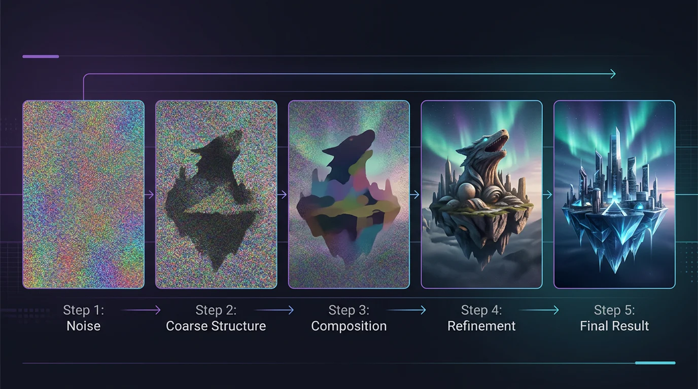
For repeatable tests, we lock the seed, checkpoint, dimensions, sampler, and steps first. Then we vary one factor. That discipline makes it possible to see whether a new prompt phrase changed the image, or whether random initialization did. For more practical walkthroughs, follow our technical videos.
Which Parameters and Controls Change the Result?
A checkpoint supplies the learned components that define the workflow’s baseline behavior. The seed sets its initial noise. Everything else either changes the denoising trajectory, changes the latent canvas, or adds a new conditioning signal.
| Control | What It Changes | Practical Trade-Off |
|---|---|---|
| Checkpoint | Base weights and compatible components | Capability, aesthetic bias, license, and controls vary |
| Seed | Initial latent noise | Supports repeatable comparison when other settings match |
| Steps | Number of denoising updates | More runtime, with diminishing returns possible |
| Sampler And Scheduler | Update rule and noise schedule | Changes speed, texture, and stability |
| Guidance Scale | Prompt-conditioned direction | Higher adherence can reduce natural variation |
| Width And Height | Latent canvas and output dimensions | More memory and compute are required |
| Positive And Negative Prompts | Text conditioning signals | Stronger constraints, not deterministic guarantees |
When Should You Add Structural Controls?
Use a control branch when the composition matters more than prompt interpretation alone. ControlNet-style conditioning can introduce processed edges, depth, segmentation, or pose information, giving the denoiser a spatial reference. The ControlNet paper demonstrates this approach across several visual control types.
Use a LoRA when you need a lightweight adaptation that modifies the behavior of a compatible base model. Use inpainting when you want to preserve most of an image while regenerating a masked region. In documented inpainting workflows, white mask areas are repainted while black areas are preserved, as the inpainting reference notes.
The safest experimentation pattern is simple: lock the base setup, change one control, save the result, and compare it against the prior run. That habit makes creative iteration measurable, and it makes failures easier to reproduce. You can join our AI community to compare notes with other builders using the same approach.
How Do You Build and Evaluate a Local Text-To-Image Workflow?
A node graph is useful because it makes the data flow visible. Instead of treating generation as a black-box button, you can inspect which component creates conditioning, which component holds the latent, and which component converts the final result into pixels.
Which Nodes Form the Core Graph?
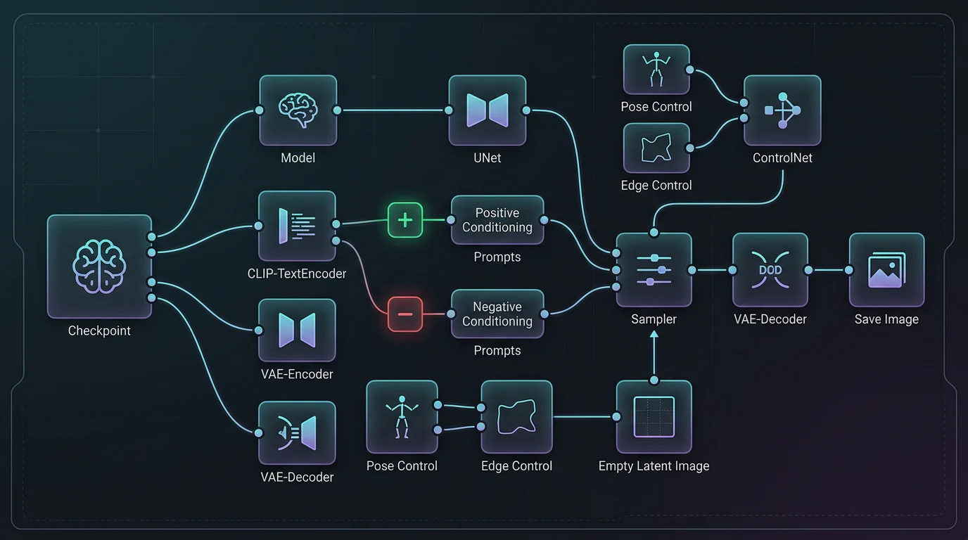
A complete local graph begins with a compatible checkpoint loader that supplies a model, text encoder, and VAE. Two text-encoding nodes create positive and negative conditioning. An empty latent node provides the canvas, then the sampler produces a cleaned latent for decoding.
Load Checkpoint
  MODEL ───────────────────────────────────────────────┐
  CLIP ──> CLIP Text Encode, Positive ─> Positive ─────┤
  CLIP ──> CLIP Text Encode, Negative ─> Negative ─────┤
  VAE ────────────────────────────────> VAE Decode     │
Empty Latent Image ─> Latent Input ────────────────────> KSampler
KSampler, Samples ────────────────────────────────────> VAE Decode → Save Image
The core node documentation confirms the same essential path: checkpoint components, text conditioning, latent sampling, VAE decoding, and image output. Read the node documentation alongside the graph, especially when a node error reveals incompatible data types.
Where Do Optional Controls Connect?
A LoRA node sits after checkpoint loading and adjusts the model and text encoder before they reach the sampler and prompt encoders. A control branch loads a control model, accepts a processed reference image, and modifies positive and negative conditioning before sampling.
For inpainting, replace the empty latent input with an image and mask encoded for editing. The rest of the loop stays recognizable: condition the sampler, generate a latent, decode it, inspect it, and save the settings that produced it.
What Should Designers Learn Before Building?
- Python And Tensors: Learn arrays, tensor shapes, basic image preprocessing, and how model inputs move between CPU and GPU memory.
- Model Inference: Understand tokenizers, text encoders, denoisers, VAEs, schedulers, and the component compatibility rules behind them.
- GPU Memory: Test dimensions, batch size, precision, and model loading choices before assuming a workflow is broken.
- Evaluation: Build a fixed prompt set, record seeds and settings, then assess adherence, composition, artifacts, latency, and repeatability.
- Licensing And Provenance: Review model terms, document sources, and preserve settings, inputs, and disclosures for every published asset.
- Deployment: Design for moderation, failure handling, observability, cost controls, and human review where the outcome can affect people.
The NIST profile treats generative AI risk as a lifecycle concern, which is why we include safety and evaluation in the first build rather than the final release. For structured media history, the C2PA specification describes signed provenance records that can support transparency.
How Should You Troubleshoot a Workflow?
| Symptom | Likely Layer | First Check | Productive Next Step |
|---|---|---|---|
| Prompt Is Ignored | Conditioning Or Guidance | Confirm both conditioning edges reach the sampler | Check types, then test moderate guidance changes |
| Composition Drifts | Weak Constraint Or New Seed | Lock the seed and simplify the prompt | Add a spatial control branch |
| Output Looks Overprocessed | Guidance, Sampler, Or Steps | Compare a lower-guidance run with the same seed | Change one parameter at a time |
| GPU Runs Out Of Memory | Dimensions, Batch, Or Precision | Record model, dimensions, batch, and error | Lower the workload or use supported memory options |
| Nodes Fail To Connect | Component Compatibility | Check checkpoint family and node data types | Use matching VAE, control, and adaptation components |
| Rights Are Unclear | License Or Provenance | Read the model card and source terms | Preserve a settings log and disclosure record |
We recommend keeping every experiment small enough to explain. That is how designers become system builders, not just skilled users of a polished interface. To continue practicing, explore learning resources.
How Vision Board Helps You Build with Generative AI
At Vision Board, we teach generative AI as a system you can inspect, test, and improve, not a prompt lottery. Our learning path connects visual intuition to the working parts that matter: Python, tensors, model inference, GPU limits, node graphs, evaluation, licensing, provenance, and deployment. We help learners turn a local workflow into a repeatable practice by recording checkpoints, prompts, seeds, controls, failures, and decisions. That discipline matters whether you are designing interfaces, automating production assets, or preparing to build image features into a product. Start with one small graph, keep a controlled experiment log, and learn why each node exists before adding another. Use our feedback loops to expose weak prompts, mismatched components, and missing safety decisions before they become costly production problems. When you are ready to deepen the work, bring your questions, test cases, and drafts to Vision Board
FAQs on Text-to-image Generation Workflow
How Does Text Become an AI-Generated Image?
Tokenized prompt text becomes conditioning embeddings. A model begins with latent noise, iteratively denoises it under that conditioning, and decodes the final latent representation into pixels.
How Do Diffusion Models Turn Noise into Images?
A denoiser receives a noisy latent and a timestep, predicts removable noise or a related residual, and a scheduler updates the latent until the VAE produces pixels.
What Happens Inside a Text-To-Image Generator?
A tokenizer and text encoder produce conditioning embeddings, a sampler initializes latent noise, a denoiser iterates with guidance, and a VAE decodes the final image.
How Do Text Embeddings Guide Image Generation?
Embeddings are supplied through attention during sampling. They steer each noise prediction toward visual patterns associated with the prompt, while guidance controls how strongly that steering applies.
What Should Designers Learn to Build Generative AI Image Tools?
Learn Python, tensors, inference, GPU memory, licensing, provenance, evaluation, and deployment. Then practice reproducible experiments that record model components, prompts, seeds, controls, outputs, failures, and decisions.